How to save RGB images using PyLibTiff

In the previous post I showed how to read and write tiff files in Python using PyLibTiff. Here I will illustrate how to use PyLibTiff to create an RGB tiff file.

The PyLibTiff on-line documentation is minimal, so I started off by simply trying to save a list containing three numpy.arrays. This was a guess based upon how I would have liked the package to work.

>>> import numpy as np
>>> from libtiff import TIFF
>>> r = np.ones((50,50), dtype=np.uint8) * 30
>>> g = np.ones((50,50), dtype=np.uint8) * 90
>>> b = np.ones((50,50), dtype=np.uint8) * 120
>>> tiff = TIFF.open('initial-test.tiff', 'w')
>>> tiff.write_image([r, g, b])
>>> tiff.close()

To my surprise this created a tiff file without complaining. However, inspecting the tiff file using exiftool revealed that the file only had one channel per sample.

$ exiftool initial-test.tiff 
...
Bits Per Sample                 : 8
Compression                     : Uncompressed
Photometric Interpretation      : BlackIsZero
...

I had in fact produced a multi-page tiff file. After some head scratching I started digging around in PyLibTiff’s built in documentation using pydoc. This was very informative. It revealed that the write_image() function has an argument named write_rgb, which by default is set to False; so I set it to True.

>>> tiff = TIFF.open('rgb-test.tiff', 'w')
>>> tiff.write_image([r, g, b], write_rgb=True)
>>> tiff.close()

Inspecting the new file revealed that it was indeed a RGB tiff file!

$ exiftool initial-test.tiff 
...
Bits Per Sample                 : 8 8 8
Compression                     : Uncompressed
Photometric Interpretation      : RGB
...

How is this useful?

Microscopy data often contains several channels of information, red and green fluorescence are common, so it is useful to be able to save these to the red and green channels respectively.

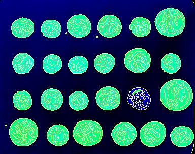
Furthermore, it can be a quick and dirty way of annotating regions of interest. Say for example that we wanted to visualise how a segmentation using the Canny edge detection algorithm followed by a binary filling of holes works in the context of the raw data. This can be achieved using the code snippet below, which was used to produce the image at the top of this post.

>>> from skimage import data
>>> from skimage.filter import canny, sobel
>>> from scipy.ndimage import binary_fill_holes
>>> coins = data.coins()
>>> edges = np.array(canny(coins), dtype=np.uint8) * 255
>>> filled = np.array(binary_fill_holes(edges), dtype=np.uint8) * 255
>>> tiff = TIFF.open('canny-fill-holes-segmentation.tiff', 'w')
>>> tiff.write_image([edges, filled, coins], write_rgb=True)
>>> tiff.close()